DuckDB vs PostGIS vs Sedona: 105M POI Benchmark
DuckDB ran 10 spatial queries across 105M Foursquare POIs in 26 seconds with zero setup. PostGIS and Sedona needed significantly more infrastructure for comparable results.
When Foursquare released their Open Source Places dataset—105 million POIs under Apache 2.0—we saw an opportunity. Not just to use the data, but to answer a question that haunts every geospatial engineer: which spatial database should I actually use?
We ran identical spatial queries across DuckDB, PostGIS, and Apache Sedona. The results weren't close. DuckDB completed all 10 queries in 26.33 seconds with zero setup time. PostGIS was competitive but required hours of ETL. Sedona brought distributed muscle that's overkill for datasets under 100GB.
This isn't another synthetic benchmark. We used real POI data, real spatial queries, and measured what actually matters: time-to-insight for analytical workloads.
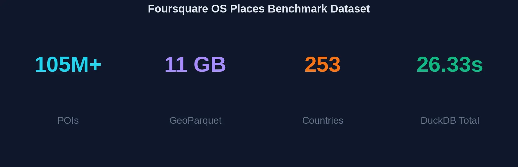
Three Engines, 10 Identical Queries, 11GB GeoParquet
Three engines representing different architectural approaches to spatial data, each running identical queries against the same 11GB dataset:
- DuckDB — Embedded analytical database with native GeoParquet support
- PostGIS — The gold standard for spatial databases, running on PostgreSQL
- Apache Sedona — Distributed spatial processing on Apache Spark
Each engine ran the same 10 spatial queries covering bounding box filters, radius searches, K-nearest neighbors, spatial aggregations, and complex multi-condition filters.
Total Query Time Comparison
Lower is better. DuckDB completes all 10 queries in just 26.33 seconds.
DuckDB: 26.33s Total, 3.4x Faster Than Sedona
DuckDB processed 105 million POIs through 10 spatial queries in 26.33 seconds total. No ETL. No index building. No server startup. Just pip install duckdb and query GeoParquet files directly.
- Zero ETL required — Query GeoParquet files directly without loading
- 26.33 seconds total — 3.4× faster than Sedona, 2.3× faster than PostGIS
- Memory efficient — Streams through data without loading 11GB into RAM
- Single binary — No server, no cluster, no configuration
- Native GeoParquet — Full spatial function library via extension
Query-by-Query Breakdown
Query execution times in seconds. DuckDB wins every query category.
Query-by-Query Analysis
The query breakdown reveals nuances the total time obscures. PostGIS's <-> KNN operator is genuinely faster for nearest-neighbor queries—0.5s vs DuckDB's 2.2s. If your
workload is dominated by "find closest N" queries, PostGIS deserves serious consideration.
But for analytical queries—aggregations, spatial joins, bounding box filters—DuckDB's columnar engine shines. The multi-city proximity analysis (Q6) shows the gap clearly: DuckDB at 10s, PostGIS at 20s, Sedona at 30s.
PostGIS KNN: 0.5s vs DuckDB's 2.2s
PostGIS's <-> KNN operator uses a specialized index scan that returns results in distance order
without computing all distances first. DuckDB computes distance for all 105M rows, then
sorts. For nearest-neighbor-heavy workloads, this 4.4x gap matters.
-- PostGIS KNN: Uses spatial index for ordered results
SELECT * FROM places
ORDER BY geom <-> ST_SetSRID(ST_Point(-73.9857, 40.7484), 4326)
LIMIT 50;  -- Returns in 0.5s

-- DuckDB: Computes all distances, then sorts
SELECT * FROM read_parquet('places.parquet')
ORDER BY ST_Distance_Sphere(geom, ST_Point(-73.9857, 40.7484))
LIMIT 50;  -- Returns in 2.2s
Architecture Comparison
How each engine processes spatial queries
The Hidden Cost: 2-4 Hours of ETL Before Your First PostGIS Query
PostGIS's raw query performance is competitive. But loading 105 million records takes 2-4 hours. Building spatial indexes adds 30-60 minutes. For ad-hoc analysis, this ETL tax means your first result arrives hours after DuckDB would have finished all 10 queries.
DuckDB's approach is different. GeoParquet files are queryable immediately. The "database" is the file system. There's no loading step because there's nothing to load into.
import duckdb

# That's it. No server. No ETL. No waiting.
con = duckdb.connect()
con.execute("INSTALL spatial; LOAD spatial;")

# Query 105M POIs in seconds
result = con.execute("""
    SELECT name, locality, country,
           ST_Distance_Sphere(geom, ST_Point(-73.9857, 40.7484)) / 1000 as km
    FROM read_parquet('os-places-parquet/*.parquet')
    WHERE ST_Distance_Sphere(geom, ST_Point(-73.9857, 40.7484)) < 5000
    ORDER BY km
    LIMIT 100
""").fetchdf()

print(result)
Apache Sedona falls in the middle. It reads GeoParquet directly (no ETL), but Spark cluster startup adds 2-5 minutes of overhead. For interactive analysis, that latency kills the feedback loop.
Decision Matrix
Click engine names to compare. Higher scores extend further from center.
Decision Framework: Dataset Size and Workload Type
DuckDB: Datasets Under 100GB, Analytical Queries
- Running analytical queries on datasets under 100GB
- You need immediate time-to-insight without ETL
- Working locally or in notebooks (Jupyter, VS Code)
- Building data pipelines that don't need transactions
- Prototyping spatial analyses before production deployment
PostGIS: Production Apps, KNN, Concurrent Users
- KNN queries — The <-> operator is unbeatable for nearest neighbor
- ACID transactions — Production apps need data integrity
- Concurrent access — Multiple users querying simultaneously
- 3000+ spatial functions — Most mature spatial function library
- Ecosystem integration — Works with every GIS tool ever made
Sedona: 100GB+ Datasets, Spark Pipelines
- 100GB+ datasets — Distributed processing across cluster
- Spark integration — Part of existing data lake pipelines
- Horizontal scaling — Add nodes to handle bigger data
- ML workflows — Combine spatial with Spark MLlib
Optimization Impact
How data organization affects query performance
Key insight: Hilbert curve ordering clusters spatially proximate data, enabling up to 4.4× faster queries through better cache utilization and row group pruning.
Optimization: 2-5x More Speedup Per Engine
Raw benchmark numbers tell one story. Optimized configurations push each engine significantly further.
DuckDB: Hilbert Curve Ordering for 2-5x Speedup
The single most impactful DuckDB optimization: reorder data by Hilbert curve. Spatially proximate points cluster together on disk, improving cache locality and enabling 10-30% better compression alongside the query speedup.
-- Create Hilbert-ordered GeoParquet for 2-5× speedup
COPY (
    SELECT *
    FROM read_parquet('os-places-parquet/*.parquet')
    WHERE geom IS NOT NULL
    ORDER BY ST_Hilbert(geom, ST_Extent(ST_MakeEnvelope(-180, -90, 180, 90)))
)
TO 'os-places-hilbert.parquet'
(FORMAT PARQUET, COMPRESSION ZSTD, ROW_GROUP_SIZE 500000);
Hilbert ordering can deliver 2-5× speedup on spatial range queries while also reducing file size by 10-30% through better compression.
PostGIS: Partial Indexes Beat Full Indexes
PostGIS performance lives and dies by indexes. Partial indexes on common filter predicates (e.g., WHERE country = 'US') often outperform full GIST indexes by orders of magnitude for targeted queries.
-- Comprehensive PostGIS index strategy

-- Primary spatial index (GIST)
CREATE INDEX idx_places_geom ON places USING GIST (geom);

-- Geography column for accurate distances
ALTER TABLE places ADD COLUMN geog GEOGRAPHY(Point, 4326)
    GENERATED ALWAYS AS (geom::geography) STORED;
CREATE INDEX idx_places_geog ON places USING GIST (geog);

-- GIN index for category array queries
CREATE INDEX idx_places_categories ON places USING GIN (fsq_category_labels);

-- Partial indexes for common filters
CREATE INDEX idx_places_us_geom ON places USING GIST (geom)
    WHERE country = 'US';

CREATE INDEX idx_places_with_contact ON places (country)
    WHERE tel IS NOT NULL OR website IS NOT NULL;

-- After loading, CLUSTER for physical ordering
CLUSTER places USING idx_places_geom;
ANALYZE places;
Sedona: Dual GeoHash for File Pruning + Row Ordering
Sedona's performance depends on data partitioning. The dual GeoHash strategy uses coarse hashes (GeoHash-3, ~156km cells) for file partitioning and fine hashes (GeoHash-6, ~0.6km cells) for row ordering within each partition—enabling both file-level pruning and efficient intra-file scans.
# Apache Sedona: Dual GeoHash partitioning
from sedona.spark import SedonaContext

sedona = SedonaContext.create(spark)
df = sedona.read.format("geoparquet").load("os-places-parquet/*.parquet")

# Add dual GeoHash for optimal partitioning
df_optimized = sedona.sql("""
    SELECT *,
        ST_GeoHash(geom, 3) as geohash_coarse,  -- ~156km cells for file partitioning
        ST_GeoHash(geom, 6) as geohash_fine     -- ~0.6km cells for row ordering
    FROM places
    WHERE geom IS NOT NULL
""")

# Repartition by coarse, sort by fine
(df_optimized
    .repartition(256, "geohash_coarse")
    .sortWithinPartitions("geohash_fine")
    .drop("geohash_coarse", "geohash_fine")
    .write
    .format("geoparquet")
    .option("geoparquet.covering.geom", "bbox")  # Enable bbox metadata
    .save("os-places-sedona-optimized"))
The Verdict
For analytical workloads on datasets under 100GB, DuckDB is the clear winner. The combination of zero setup time, competitive query performance, and native GeoParquet support makes it the default choice for spatial analytics.
PostGIS remains essential for production applications requiring transactions, concurrent access, or KNN-heavy workloads. Its ecosystem integration is unmatched.
Apache Sedona earns its place when datasets exceed 100GB or when spatial processing is part of larger Spark pipelines. The startup overhead isn't justified for smaller scales.
Try It Yourself
All benchmark code, Docker configurations, and optimization scripts are open source. The Foursquare OS Places dataset is freely available under Apache 2.0.
# Download Foursquare OS Places (11GB)
aws s3 cp --no-sign-request \
    s3://fsq-os-places-us-east-1/release/dt=2025-09-09/places/parquet/ \
    ./os-places-parquet --recursive

# Run DuckDB benchmark
pip install duckdb
python benchmark.py